⚡️ TL;DR
In this post, we delve into Big O Notation, a fundamental concept in computer science used to describe the efficiency of algorithms. We’ll explore how Big O helps in analyzing time complexity and provide examples to illustrate its application.
In general, we can’t simply label one algorithm a 400-ste algorithm and another a 500-step algorithm. This is because the number of steps an algorithm takes cannot be pinned down to a single number. Let’s take linear search, for example. The number of steps it takes to find an element in a list depends on the position of the element in the list. If the element is at the beginning of the list, the algorithm will take fewer steps than if the element is at the end of the list.
The more effective way, then, to quantify the efficiency of linear search is to say that linear search takes N steps to find an element in a list of N elements. This is a more general way to describe the efficiency of an algorithm.
To help ease communication regarding time complexity, computer scientists have borrowed a concept from mathematics to describe a concise and consistent language around the efficiency of data structures and algorithms. Known as Big O Notation, this formalized expression of these concepts allow us to easily categorize the efficiency of a given algorithm and convey its efficiency to others.
What is Big O Notation?
Once you understand Big O Notation, you’ll have the tools to analyze each algorithm you encounter and determine its efficiency. Let’s start applying Big O to the algorithm of linear search.
In a worst case scenario, linear search will take as many steps as there are elements in the array. For N elements in the array, linear search can take up to N steps. This is expressed in Big O Notation as O(N).
Here’s what the notation means. It expresses the answer to what we’ll call the key question: if there are N data elements, how many steps will the algorithm take in the worst case scenario? Go ahead and read the sentence again, but this time replace the N with the number of elements in the array. This is the essence of Big O Notation.
Let’s contrast this with how Big O would express the efficiency of reading from a standard array. Reading from an array takes just one step, no matter how large the array is. To figure out how to express this in Big O terms, we are asking the same key question: if there are N data elements, how many steps will the algorithm take in the worst case scenario? In this case, the answer is always 1. So, the Big O Notation for reading from an array is O(1).
O(1) is interesting, since all algorithms that take a constant number of steps to complete are considered to be O(1). This is because the number of steps the algorithm takes does not depend on the number of elements in the array. This is the most efficient time complexity an algorithm can have.
The soul of Big O Notation
Now that we understand O(N) and O(1), we begin to see that Big O Notation does more than simply describe the number of steps an algorithm takes. Rather, it’s an answer to that key question: if there are N data elements, how many steps will the algorithm take in the worst case scenario?
Let’s say we have an algorithm that takes three steps no matter how much data there is. That is, for N elements, the algorithm always takes three steps. In Big O terms, this is O(3). But, since the number of steps the algorithm takes does not depend on the number of elements in the array, we can simplify this to O(1).
The soul of Big O is what Big O is trying to tell us. It’s not just about the number of steps an algorithm takes, but about how an algorithm’s performance changes as the data changes.
an algorithm that is O(N), on the other hand, is a different type of algorithm whose performance changes linearly with the data. If the data doubles, the number of steps the algorithm takes also doubles. This is the story O(N) tells us. It tells about the proportional relationship between the data and the algorithm’s efficiency. It describes exactly how the number of steps increases as the data increases.
Deeper into the Big O
Say we had an algorithm of constant time that always took 100 steps no matter how much data there was. Would you consider that to be more or less performant than an algorithm that is O(N)?
For a data set that is fewer than 100 elements, an O(N) algorithm takes fewer steps than the O(1) 100-step algorithm. But, as the data set grows, the O(N) algorithm will eventually surpass the O(1) algorithm in terms of efficiency. This is the power of Big O Notation. It allows us to compare the efficiency of algorithms as the data changes.
Because there will always be some amount of data at which the tides turn, and O(N) takes more steps from that point until infinity, O(N) is considered less efficient than O(1) no matter how many steps the O(1) algorithm takes.
An algorithm of the third kind
Let’s now look at how to describe binary search in terms of Big O Notation. We cannot describe it as O(1). because the number of steps increases as the data increases. It also doesn’t fit into the category of O(N), since the number of steps is much fewer than the N data elements. So, how do we describe binary search?
Binary search is an algorithm that takes log(N) steps to find an element in a sorted array of N elements. This is because binary search cuts the data in half with each step. This is the most efficient time complexity an algorithm can have, and it is expressed in Big O Notation as O(log(N)). This way describes that the number of steps the algorithm increases one step each time the data is doubled.
In computer science, whenever we say O(log N), it’s actually shorthand for saying O(log2 N). This is because the base of the logarithm doesn’t matter when we’re talking about Big O Notation. The base of the logarithm is a constant, and Big O Notation is only concerned with the growth rate of the algorithm.
Speeding up our code with Big O
With Big O, we also have the opportunity to compare our algorithm to general algorithms out there in the world, and assess Is this a fast or slow algorithm as far as algorithms generally go?
But what if we might be able to modify the algorithm in order to give it a nice efficiency bump?
Bubble Sort
Let’s look at a new category of algorithmic efficiency using one of the classic algorithms of computer-science. Sorting algorithms have been the subject of extensive research and tens of them have been developed over the years all solve the same problem: given an array of unsorted values, how can we sort them so that they end up in ascending order?
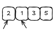
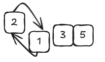
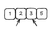
Bubble Sort is a very basic sorting algorithm and follows these steps:
- Point two consecutive values in the array and compare the first item with the second.

- If the two items are out of order (the left is greater), swap them. If they already happen to be in the correct order, do nothing.

- Move the pointers one cell to the right.

- Repeat steps 1-2-3 until we reach the end of the array. At this point, we have completed our first pass-through of the array by pointing to each of its values until we reach the end. We then move the two pointers back to the first two values of the array and execute another pass-through of the array. We keep on executing these pass-throughs until we did not perform any swaps. It means our array is fully sorted.
- The reason why this algorithm is called Bubble Sort is easy: in each pass-through, the highest unsorted value “bubbles” up to its correct position. BAsically every time we perform a pass-through with some swap we need to do an additional one up to there are none swaps.
Here’s an implementation in code:
 1func BubbleSort(arr []int) []int {
 2   // We define a variable to keep track of whether we swapped any elements in the last iteration
 3   swapped := true
 4
 5
 6   // We will continue to iterate through the array until no elements are swapped
 7   for swapped {
 8       // We set the swapped variable to false at the beginning of each iteration
 9       swapped = false
10
11
12       // We iterate through the array, comparing each element with the next one
13       for i := 0; i < len(arr)-1; i++ {
14           // If the current element is greater than the next element, we swap them
15           if arr[i] > arr[i+1] {
16               arr[i], arr[i+1] = arr[i+1], arr[i]
17               // We set the swapped variable to true to indicate that we swapped elements
18               swapped = true
19           }
20       }
21   }
22
23
24   // We return the sorted array
25   return arr
26}
The Efficiency of Bubble Sort
This sort algorithm has two significant kinds of steps: comparisons to determine which is greater and swaps to change the position.
Let’s see how many comparisons take place in Bubble Sort.
In our example of four elements, we have to make three comparisons between sets of two numbers, in our second pass-through, only two because we don’t need to compare the final two numbers since it was in the correct spot due to the first pass-through.
So that’s: 3+2+1=7 comparisons. To put this in a way for N elements we make (N-1)+(N-2)+…+1 comparisons
Now let’s analyze the swaps.
In a worst case scenario, where the array is sorted in descending order, we need a swap for each comparison so we would need 7 comparisons and 7 swaps for a grand total of 14 steps.
Let’s look at the big picture. With an array containing 20 values we’d have: 19+18+17+16+15+14+13+12+11+10+9+8+7+6+5+4+3+2+1=190 comparisons and 190 swaps for a total of 380 steps.
As the number of elements increases, the number of steps grows exponentially, in math terms, it grows approximately quadratically as seen in the following table:
| Data elements | Max # of steps | N² |
|---|---|---|
| 5 | 20 | 25 |
| 20 | 380 | 400 |
| 25 | 40 | 625 |
| 20 | 1560 | 1600 |
Expressing it with Big O Notation we need to answer the key question: if there are N data elements, how many steps will the algorithm take?
O(N²) is considered to be a relatively inefficient algorithm since as the data increases, the steps increase dramatically. It is also referred to as quadratic time.
The quadratic problem
Let’s say we are working on a Go application that analyzes the ratings given to products, where users leave ratings from 1 to 10 and we need to write a function that checks whether an away of ratings contains any duplicate numbers. This will be used in moe complex calculations in other parts of the software,
On the first approaches that may come to mind is the use of nested loops:
While this certainly works, is it efficient? Applying Big O to our situation, we’d ask ourselves: for N values in teh array provided to our function, how many steps would our algorithm take in a worst-case scenario?
In a worst-case scenario, the array contains no duplicates, which would force our code to complete all of the loops and exhaust every possible comparison before returning false. We can conclude that for N values in the array, our function would perform N² comparisons. For each iteration, we must iterate another N times in our inner loop.
Very often (but not always), when an algorithm nests one loop inside another, the algorithm is O(N²). So whenever you see a nested loop, O(N²) alarm bells should go off in your head.
A linear solution
Following is another implementation that doesn’t need nested loops. It creates an array prior to the loop which starts out empty.
Then, we use a loop to check each number in the array. As it encounters each number, it places a true in the array at the index of the number we are encountering.
For example; let’s say our array ir [3,5,8] so at the end of the algorithm we will have [false, false, false, true, false, true, false, false, true]
Now, here is the real trick. Before the code stores a true in the appropriate index, we check first that the index already has a true as its value. If it does, this means we have already found that number, meaning we found a duplicate. We simply return true and cut the function short.
In terms of worst-case scenario, such a scenario would occur when the array contains no duplicates, in which case our function ust complete the entire loop.
This new algorithm makes N comparisons for N data elements, then, is O(N). We know that this O(N) is much faster than O(N²) su by using this second approach we have optimized our function significantly. This is a huge speed boost.
There is actually one disadvantage with this new implementation since it will consume more memory than the first one. We need to deal with space constraints, but that will be covered in another post.